Amazing skating rinks

21

The board moves on round rollers. At the same time, it maintains a horizontal position and remains at the same height. Why is this happening? Yes, because the circle has the same width no matter how it turns.

Will the dock move the same way if you use non-circular rollers? At the first moment it seems that this is impossible. Let’s not rush, however. It turns out that there are curves that, like a circle, have the same width in all directions. They are called lines of the same width.

One of the simplest curves of this kind is shown in figure 1. It consists of two $A_1B_1, A_2B_2, A_3B_3$ of radius $r$ and two $B_1A_3, B_3A_2, B_2A_1$ of radius $R$, the centers of which are located at the vertices of a regular triangle $O_1O_2O_3$. It is easy to see that the width of this curve is the same in all directions and is equal to $R+r$. Consequently, rollers whose profiles are sequential along such curves will work no worse than round ones (Fig. 2).

The curve shown at figure 1 can be obtained as follows. Let’s take the segment $A_1B_3$ and rotate it by $60^\circ$ around the point $O_1$ and move it to position $B_1A_2$. Then, rotate the segment $B_1A_2$ by $60^\circ$ around the point $O_2$, we get the segment $A_3B_2$ and, finally, rotate the segment $A_3B_2$ by $60^\circ$ around the point $O_3$, again we arrive at the segment $A_1B_3$. In the process of these turns, one end of the segment is considered, arcs $A_1B_1A_3B_3$, and the other - arcs $B_3A_2B_2A_1$. Therefore, the curve shown in figure 1 can be considered as a trajectory described by the ends of some

22

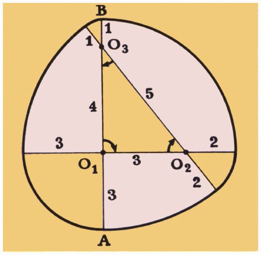
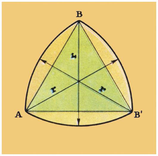
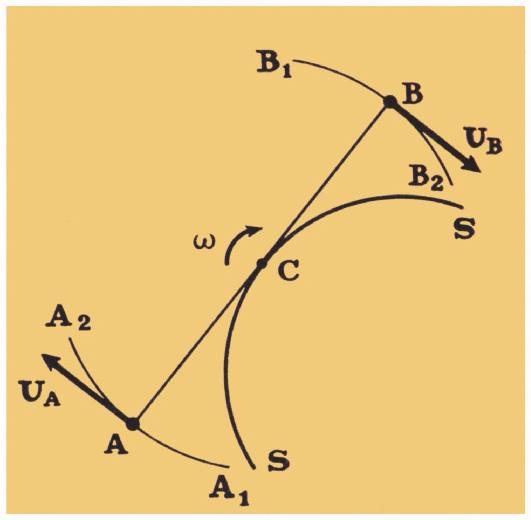
Fig. 3.

The width of all these curves is constructed and is equal to the length of the rotated segment. You can rotate a segment around one of its ends. This way we get the simplest curve of equal width, different from a circle (Fig. 4). In this case, the segment $AB$ rotates first around the point $A$, moving to the position $AB'$, then around the point $B'$, passing into the segment $B'B$, and, finally, around the point $B$, closing the curve.

Let us now consider the non-actor segment $AB$. Let it roll without sliding along the SS curve. Then in every

Fig. 4.

In a separate moment, such movement can be considered as rotation of a segment relative to the point of contact. The tangent point about which the rotation is currently being made is called the instantaneous center of rotation (for example, point $C$ on figure 5).

The idea of ​​an instantaneous center of rotation makes it easy to calculate the velocities of various points on the segment $AB$. For example, for the speed of points $A$ and $B$ we have

$$v_A = \omega \cdot CA,$$
$$v_B = \omega \cdot CB,$$

where $\omega$ is the angular velocity of the segment $AB$ in its “instantaneous” rotation around the center $C$. In this case, the velocities of the points under consideration will be perpendicular to the corresponding radius of rotation, that is, the segments $CA$ and $CB$. In this way, you can calculate the speed of any point lying on this segment or rigidly connected with this segment. If, for example, a non-actor figure is rigidly connected to the segment $AB$, then the speed of any point $P$ is equal to the product $\omega \cdot CP$.

Let us now return to the constructed width curves. Let the segment $AB$ roll along the curve SS. Since the velocities $v_A$ and $v_B$ are perpendicular to the radii $CA$ and $CB$, they are parallel to each other. But the speed $v_A$ is directional

23

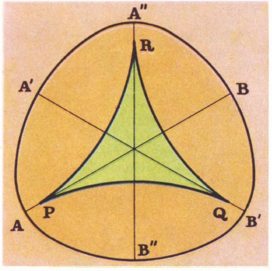
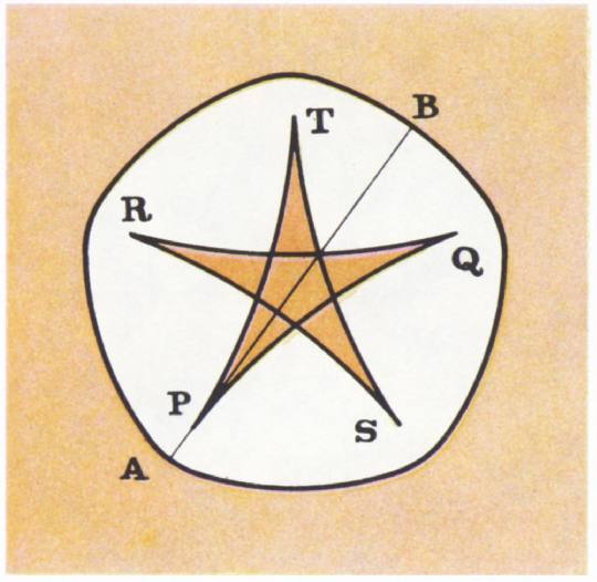
Fig. 6.

line is tangent to the trajectory of point $A$, and speed $v_B$ is tangent to the trajectory of point $B$. Therefore, these tangents are parallel to each other, and the distance between them remains equal to $AB$ all the time. But this means that the trajectories $A_1A_2$ and $B_1B_2$ can be considered as parts of some curve of constant cyrin.

However, we need to construct not two sections, but just this curve. If we want to do this using the described operation, we must choose the line $SS$ so that, by drawing it, the segment $AB$ rotates to $180^\circ$, that is, so that the point $A$ comes to the position $B$, and the point $B$ to the position $A$. However, of such lines - $PQRP$ - is shown on figure 6. Let us trace in more detail how the segment $AB$ describes it.

First it rolls along area $PQ$ and comes to position $A'B'$. Moreover, its ends describe the arcs $AA'$ and $BB'$. Then it rolls along the section $QR$, and its ends describe the arcs $A'A''$ and $B'B''$. Finally, it marks the part $RP$, and its ends move along the arcs $A''B$ and $B''A$. As a result, point $A$ comes to position $B$, and point $B$ to position $A$, and the curve of the constructed cirina is closed. In this case, arcs $PQ$, $QR$

and $RP$ can have any shape and do not have to be the same. The only thing that is required of them is that they be convex and touch each other as shown in figure. As for the segments $AP$ and $PB$, their length cannot be arbitrary, or then the arc described by the point $A$ will not “join” the arc described by the point $B$. Here you can build as follows. Let us draw a straight line through the point $P$, tangent to the arc $PQ$, and place the point $A$ on it. Let us now force this straight line to line $PQRP$. Then the end of the arc, which will cover the point $A$, determines the position of the point $B$.

Line $PQRP$, shown in figure 6, consists of three arcs. But the number of arcs may be greater. For example, on figure 7 the curve of the constructed tsirina is shown, obtained by drawing the line $PQRSTP$, consisting of the heel of the arcs.

The curves of the constructed cirina have one more property that makes them similar to the circle. They are expressed by the following theorem:

The perimeter of the curve of the constructed cirina is $l=\pi D$, where $D$ is the width of this curve.

Let’s prove this theorem.

24

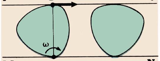
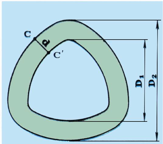
Fig. 8.

Let the horizontal straight line $PQ$ be moved using rollers of constant width (Fig. 8). In the distance is one of these skating rinks, for example the left one. Let its width be $D$ and its perimeter be $l$. When the straight line $PQ$ moves so much that this roller makes one revolution, it moves relative to the straight line $MN$ by a distance $l$ to the right. But since it rolls not only along the straight line $MN$, but also along the straight line $PQ$, then after one revolution it turns out to be folded relative to the straight line $PQ$ by a distance $l$ to the left. Consequently, the displacement of straight line $PQ$ relative to straight line $MN$ will be equal to $2l$.

But since this same mixing is equal to $vt$, where $t$ is the time during which the roller makes one revolution, then

$$2l = vt. \tag{1}$$

(We assume that straight line $PQ$ moves at a constant speed.) The instantaneous center of rotation of the roller is at point $A$, which means that the speed of movement

$$v = \omega \cdot AB = \omega D,$$

where $\omega$ is the angular speed of the roller. Substituting this expression into equality (1), we obtain

$$2l = \omega Dt. \tag{2}$$

But $\omega t$ is the angle of rotation of the roller per revolution. Hence,

$$\omega t = 2\pi,$$

and equality (2) takes the form

$$2l = 2\pi D,$$

where

$$l = \pi D.$$

Thus, the perimeter of a constant width curve is calculated in the same way as the perimeter of a circle. What is the area enclosed by a curve of constant width? Can it be calculated in the same way as the area of ​​a circle? It turns out not. However, the area of ​​a scapula of constant width can be calculated as the area of ​​the scapula between two concentric circles. More precisely this means the following.

Consider a curve of constant width (Fig. 9). Through an arbitrary point $C$ we draw a normal on it (a straight line perpendicular to the tangent is normally called) and plot a segment $CC'$ of a given length $d$ along it. By setting aside such segments from each point of a given curve, we obtain a new curve, which is the geometric locus of the ends of the delayed segments. Obviously, it will also have a constant width. If we now denote by $S$ the area enclosed between these curves, then the equality will be true

$$S = \frac{\pi D_2^2}{4} - \frac{\pi D_1^2}{4},$$

where $D_1$ is the width of the inner curve, and $D_2$ is the width of the outer one.

Try to prove it yourself.