Solutions to problems M70—M73; F79—F82

26

In this issue we publish the solution to problems M70–M73

M70

Let $l_1, l_2, \dots, l_n$ be several lines in the plane, among which there are two intersecting lines. Prove that it is possible, and in a unique way, to choose on each of these lines at the point $X_1, X_2, \dots, X_n$ so that the redistribution restored at the point $X_i$ to the line $l_i$ passes through the point $X_{i+1}$ (for all $i=1, 2, \dots, n-1$), and the redistribution restored to $l_n$ at the point $X_n$ passes through the point $X_1$.

Try to formulate and prove a similar theorem in space.

This problem can also be formulated as follows. Let $p_i$ be a mapping that assigns to each point $M$ (on the plane) its projection onto the line $l_i$, that is, $p_i(M)$ is the base of the redistribution dropped from the point $M$ to the line $l_i$. It is required to prove that on the line $l_1$ there is a unique point $X_1$ such that after $n$ mappings

$$X_1 \xrightarrow{p_n} X_n \xrightarrow{p_{n-1}} X_{n-1} \xrightarrow{p_{n-2}} \dots$$

turns into itself.

For an arbitrary point $X$ of the line $l_1$ denotes through $f(X)$ the point on the line $l_1$ at which it passes

$$X$$ after $n$ mappings $p_n, p_{n-1}, \dots, p_1$ (Fig. 1); it is written like this:

$$f = p_1 \circ p_2 \circ \dots \circ p_n.$$

Let’s choose the origin and direction on each of our lines $l_i$, that is, we’ll turn each of them into a numerical axis (we choose the same scale unit on all lines). (We identify a point (on a line) and its corresponding number—its coordinate—so that the maps $p_1, p_2, \dots, p_n$ and $f$ can now be considered functions that

27

Each number is assigned a new number.

Let us prove that the mapping $f$ is linear: $f(x) = ax + b$.

To do this, it is enough to prove the following three obvious statements.

(1) If $l$ and $l'$ are two straight lines and $p : l \rightarrow l'$ is a map that associates each point with its projection onto $l'$, then $p$ is a linear map.

(2) If $p_1$ and $p_2$ are linear maps, then so is $p_1^\circ p_2$.

(3) If $p_1, p_2, \dots, p_n$ are linear maps, then $f = p_1^\circ p_2^\circ \dots p_n^\circ$ is also a linear map.

It is clear that (3) is derived from (2) by induction. Check (2): if $p_1(x) = a_1x + b_1$ and $p_2(x) = a_2x + b_2$, then $(p_1^\circ p_2)(x) = p_1(p_2(x)) = a_1a_2x + (a_1b_2 + b_1)$. To prove (1), check this formula:

$$p(x) = x \cos \alpha + c,$$

where $\alpha$ is the angle between the positive direction of the axes $Ox$ and $O'x'$, $c$ is the coordinate of the point $p(O)$ in the system $Ox'$ (Fig. 2; consider also the case when the lines $l$ and $l_1$ are parallel).

Now, to solve the problem, it is enough to show that the linear equation $x = ax + b$ has a solution, and only one. If this is not the case (that is, if there are no solutions or more than one), then $a = 1$. Let us prove that this cannot be. Note that with each projection $p_k$: $l_{k+1} \rightarrow l_k$ the distance between any two points does not increase:

$$|p_k(x) - p_k(x')| \leq |x - x'|,$$

and if the lines $l_{k+1}$ and $l_k$ are not parallel, then strictly decreases. It follows that for any two points $x$ and $x'$

$$|f(x) - f(x')| < |x - x'|.$$

But if $a = 1$, that is, if $f(x) = x + b$, then $f$ preserves the distances between any two points (it simply shifts them all by the distance $b$). We got a contradiction. The proof is legal.

Problem M70 and our solution have been re-established without any changes for the case when the lines are located not on a plane, but in space (they can also be intersecting). In this case, $p_k$ means projection onto the line $l_k$ in space: a mapping that corresponds to each point the base of the perpendicular dropped from this point onto the line $l_k$.

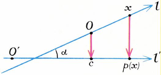
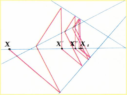
Fig. 2. A mapping that assigns to each point on one line its projection onto another line is written as a linear function.

Fig. 3. Point $X_1$, for which $f(X_1) = X_1$, it is practically easy to find a method of successive approximations: starting from an arbitrary point $X$, lower the perpendiculars to the given lines and find the successive after each “cycle” of the point $X' = f(X)$ $X'' = f(X')$ and so on. It is not difficult to prove that the distances $|X - X_1|, |X' - X_1|, |X'' - X_1|$, … form an infinite decreasing geometric progression with the value $|a| < 1$, so that by repeating the construction several times, we can find the position of the point $X_1$ with any ironclad accuracy. A similar method is very used to find a solution to an equation of the form $f(X) = X$; it will be applied when the function $f$ decreases the distance between any two points. In our case, when $f$ is a linear function, labeled, the solution to equation $f(X) = X$ can be found exactly (think about how to find the point $X_1$ if $X, X'$ and $X''$ are known).

28

There is another possibility of generalization:
look at straight planes together. Can
prove, for example, the following fact: if the data $n$
planes in space, among which
there are three intersecting at one point,
then it is possible and in the only way
select on each of these planes
point $X_k$ ($k=1, \dots, n$) so that the
ndikulier, restored at point $X_k$ to co-
corresponding plane, passed through
point $X_{k+1}$ (and $X_{n+1}=X_1$). Now it’s already
$f=p_1 \cdot p_2 \dots p_n$ will be a linear mapping
plane to plane and coordinates will be written as follows: $f(x, y)=$ $(x', y')$, where $x'=a_1x+b_1y+c_1$, $y'=a_2x+b_2y+c_2$.

Prove that if the system of equations
$$\begin{cases} x=a_1x+b_1y+c_1, \\ y=a_2x+b_2y+c_2 \end{cases}$$
has no solutions or has more than one
solutions (this happens if $(a_1-1)(b_2-1)−a_2b_1=0$), then the system $x=a_1x+b_1y$, $y=a_2x+b_2y$ has a solution $(x_0, y_0)$, different from $(0,0)$, and that the mapping $f$ does not change the dis-
standing between points $(0,0)$ and $(x_0, y_0)$, which cannot happen in our problem.

Nanmore complete solutions to the problem
Slania F. Schmidel from Moscow, Yu. Obolonkov from Voronezh, M. Rozov from Minsk.

M71

A rectangular table of $m$ rows and $n$ columns is filled with numbers. Let’s rearrange the numbers in each line in ascending order. Prove that if you then rearrange the numbers in each column in ascending order, then in each row they will still appear in ascending order.

Think about what will happen if you act in a different order: in the original table, first rearrange the numbers in ascending order in the columns, and then in the rows: will the result be the same table as in the first case or a different one?

Let’s consider a table in which in each row the numbers are in ascending order, and prove that if $l<r$, then the largest number in the $r$th column (we denote it by $b$) is not less than the largest number in the $l$th column (we denote it by $a$). Indeed, the number at the intersection of the line where $a$ is and the $r$ column is no less than $a$ (because the numbers in the line are in ascending order).

Similarly, one can prove that the $k$th largest number (counting from the largest number in the $r$-column $(b_k)$) is no less than the $k$th largest number in the $l$th column

29

Different tables are read. To verify this, it is enough to give an example (Fig. 5).

The problem was solved correctly by P. Ayulov, A. Brevdo, L. Brauzinsky, G. Vysotskaya, S. Grigoryan, A. Gordenko, I. Jabbarov, A. Kleyin, A. Kmizhnerman, I. Kochubeevsky, G. Levin, M. Preezer, E. Skryt, A. Slinkin, A. Chernyak and others. In addition to the solution, there are many others close to ours in which induction is carried out; In some works it has been proven that it is possible to rearrange each column in succession so that the numbers will always appear in the rows in ascending order.

N. B. Vasiliev

M72

Solve the equation
$$\sqrt[3]{1-x} + \sqrt[3]{1+x} = p,$$
(1)
where $p$ is an arbitrary real number.

A naive attempt at a solution: cube both sides of the equation
$$2 + 3\sqrt[3]{1-x^2}\left(\sqrt[3]{1-x} + \sqrt[3]{1+x}\right) = p^3$$
(2)
and substitute here the original equality (1):
$$2 + 3p\sqrt[3]{1-x^2} = p^3.$$ (3)
Now it’s easy to find $x$:
$$x = \pm \sqrt{1 - \left(\frac{p^3 - 2}{3p}\right)^3}.$$ (4)
We were sent many letters where this answer was received (in this and other ways). There were also quite a few letters in which it was correct to find a set of values ​​of $p$ for which formula (4) makes sense:
$$p = -1, \quad 0 < p \leq 2.$$
Some even noticed that the value $p = -1$ should be discarded, since the value $x = 0$ given by the formula $p$ is not suitable. But it was not proven that for all $p$, $0 < p \leq 2$ the value $x$ given by formula (4) are solutions. (Usually such a proof is a test, but here it is very difficult to do.) And this must be proven, since not all transformations performed above remain equivalent: equation (2) is not equivalent to (3). To see this, substitute $x = 0$, $p = -1$ in (2) and (3). Equality (3) will return to the same place, but (2) will not. Therefore, the statements found in the letters that this transformation is equivalent are incorrect. (Indeed: try to derive (2) from (3). You will have to use equality (1), the conditions of the problem, and this cannot be done, since this is precisely what needs to be proven.) If this is so, then other roots may be constructed.

Let us examine in more detail the transformations we made to the equation. Let us denote $\sqrt[3]{1-x} = u$ and $\sqrt[3]{1+x} = v$ for brevity.

From Eq.
$$u + v = p$$
we moved on to the equation
$$u^3 + v^3 + 3uv(u + v) = p^3$$
(2)
using an equivalent transformation (raising the object into a cube). The next step is to substitute $p$ together with $u + v$ and go to the equation
$$u^3 + v^3 + 3uvp = p^3,$$
(3)
which we will write like this:
$$u^3 + v^3 - p^3 + 3uvp = 0,$$
$$(u + v)^3 - p^3 - 3uv(u + v - p) = 0.$$
Let’s apply the formula for the difference of two cubes and then put $(u + v - p)$ out of brackets:
$$(u + v - p)(u^2 + v^2 + p^2 + up + pv - uv) = 0.$$ (3’)
So, we managed to write equation (3) in this form (3’), from which it is easy to study why it is not equivalent to (2). It is clear that the left side of (3’) is equal to zero when at least one parenthesis is equal to zero:

1. $u + v - p = 0,$
2. $u^2 + v^2 + p^2 + up + pv - uv = 0.$

30

The first equality is our original equation. This means that the entire construction of the solution is related to the second one and we need to find out when it is executed. Multiplying it by 2, you can write it like this:

$$(u+p)^2+(v+p)^2+(u-v)^2=0.$$

This equality holds only for $u=v=-p$.

In application to our equation:

$$\sqrt[3]{1-x}=\sqrt[3]{1+x}=-p.$$

This means that $x=0$ for $p=-1$ is the only constructed root. All other roots given by formula (4) for $0<p\leqslant2$ satisfy equation (1).

Let us write down again the identities that we have successfully established (for symmetrina we replace $p$ with $-w$):

$$u^3+v^3+w^3-3uvw=(u+v+w)(u^2+v^2+w^2-uw-vw-uv),$$

$$2(u^2+v^2+w^2-uw-vw-uv)=$$

$$=(u-v)^2+(v-w)^2+(w-u)^2.$$

They are often useful in proving inequalities and in other problems.

M73

On a lottery ticket you need to mark 8 cells out of 64. What is the probability that after a drawing in which 8 cells out of 64 are also chosen (and we consider all such possibilities to be equally probable), it turns out that exactly 4 cells are guessed? 5 cells?…all 8 cells?

As is known, 8 cells out of 64 can be chosen in $C_{64}^8=\frac{64!}{8!56!}$ ways ($n!$ is the product of all integers from 1 to $n$ inclusive) $^*$). All these methods are equally reliable. Therefore, the probability of getting any one particular way is $1/C_{64}^8$. Now we need to calculate what time the case turned out to be exactly $k$ cells ($0\leqslant k\leqslant8$). The number of such cases is equal to the number of methods

$^*$) See, for example, the article by N. Ya. Vilenkin “Combinatorics” in «Kvant» No. 1, 1971.

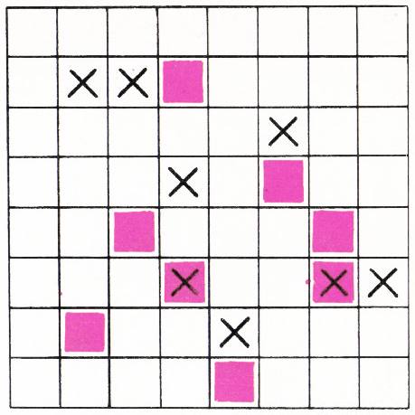
Fig. 6. Red cells are winners; The 8 cells we have selected are marked with a cross. On this figure $k=2$, $8-k=6$.

methods in which $k$ cells are selected from 8 marked and $8-k$ cells from 56 unmarked. Therefore it is equal to $C_{8}^k\cdot C_{56}^{8-k}$. To find the desired time $f_k$ - the probability of guessing exactly $k$ cells, you need to multiply the probability of one method by this number. We get

$$f_k=\frac{C_{8}^k\cdot C_{56}^{8-k}}{C_{8}^4}.$$

Thus, the probabilities of guessing 0,1, …, 8 cells are equal to the corresponding ones.

$$f_0=\frac{C_{8}^0\cdot C_{56}^8}{C_{8}^4},$$

$$f_1=\frac{C_{8}^1\cdot C_{56}^7}{C_{8}^4}, \dots, f_8=\frac{C_{8}^8\cdot C_{56}^0}{C_{8}^4}.$$

The sum of these nine numbers is, of course, equal to one.

Formally, the problem is a solution, but from a practical point of view this is not yet the case. I would like to imagine how great the chances are of guessing a particular number of cells if we buy and fill, say, ten lottery tickets. To do this, you need to approximately represent these numbers in the form of decimal fractions. This can be done using a slide rule; for example, directly use formulas (1). This is what A. Zlomnik from the city of Zhukovsky did. We will describe another, as it seems to us, simpler method.

31

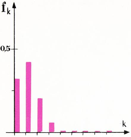
Fig. 7. Shown here are the numbers $f_k$ – the probabilities of guessing $k$ cells ($k = 0, 1, 2, \dots, 8$). At $k \geq 4$ the values ​​of $f_k$ are very close to zero.

First, let’s calculate the ratio of the $(k+1)$th of these numbers to the $k$th one:

$$\frac{f_{k+1}}{f_k} = \frac{C_8^{k+1} \cdot C_{56}^{8-k-1}}{C_{64}^8} : \frac{C_8^k \cdot C_{56}^{8-k}}{C_{64}^8} = \frac{(8-k)^2}{(k+1)(48+k+1)}$$

in part,

$$\frac{f_1}{f_0} = \frac{64}{49} \approx 1.31; \quad \frac{f_2}{f_1} = \frac{49}{100};$$

$$\frac{f_3}{f_2} = \frac{12}{51} \approx 0.235; \quad \frac{f_4}{f_3} = \frac{25}{208} \approx 0.12;$$

$$\frac{f_5}{f_4} \approx 0.06; \dots$$

By calculating the ratio of $f_2, f_3, f_4$ to $f_0$ with two decimal places:

$$\frac{f_2}{f_0} = 0.64; \quad \frac{f_3}{f_0} \approx 0.15; \quad \frac{f_4}{f_0} = 0.02.$$

It is clear that $f_5/f_0 < 0.02 \cdot 0.12$ and, for the chosen degree, exactly $f_5, f_6, f_7, f_8$ are equal to zero. We can make an equation

$$f_0(1+1,31+0,64+0,15+0,02)=1,$$

whence $f_0 \approx 0.32$. Now finding $f_1, f_2, f_3, f_4$:

$$f_1 \approx f_0 \cdot 1.31 \approx 0.42; \quad f_2 \approx f_0 \cdot 0.64 \approx 0.20;$$

$$f_3 \approx f_2 \cdot 0.24 \approx 0.047; \quad f_4 \approx f_3 \cdot 0.12 \approx 0.0056.$$

Thus, if you fill out ten tickets, then the average ones will most likely all be those on which 0, 1, 2 and, perhaps, 3 cells are guessed; The probability of guessing 4 or more cells is very low. By multiplying $f_4$ by $\frac{f_5}{f_4} \approx 0.06$ and so on, approximations of $f_5, f_6, f_7, f_8$ can be obtained. In part, $f_8 \approx 2 \cdot 10^{-10}$. This means that in order to have a real chance of guessing all 8 cells, you need to fill out several tens of billions of tickets.

Using the approximate calculation method that we applied, it can be shown that if the number of $N$ cells on a lottery ticket is much greater than the number of $m$ cells that need to be eliminated, and $m$ is sufficiently large, then the probability of guessing $k$ cells of the approximate is equal to

$$f_k = \frac{C_m^k C_{N-m}^m}{C_N^m} \approx \frac{\mu^k \cdot e^{-\mu}}{k!},$$

where $\mu = \frac{m^2}{N-2m}$ and $e \approx 2.718\dots$ is a constant number ($\pi$), so we need to use the fact that $1+x+\frac{x^2}{2}+\frac{x^3}{3!}+\dots = e^x$ for any $x$).

A. L. Toom

In this issue we publish solutions to problems F79—F82

F79

The level of water entering the boat coincides with the water level in the lake. Where will the water level be higher if you throw a log into the boat?

When lowering a log into a boat, the boat will plunge into the lake, you will receive an additional volume of water $\Delta V = \frac{m}{\rho}$ ($m$ is the mass of the log, $\rho$ is the density of water). On the other hand, since the log floats in water, the water level in the boat should change in the same way as it would change if water with a mass equal to the mass of the log and a volume equal to the volume of the immersed part of the log, that is, $V = \frac{m}{\rho}$, was added to the boat. (We can mentally remove the log and fill the resulting water with water, but the water level in the boat will not change.) The same volume of water additionally flows out from the boat when the log is thrown into it. Therefore, the water level in the boat will be the same as the water level in the boat.

32

low water in the lake if the thickness of the walls of the boat is negligible, and will be slightly higher than the water level in the lake if the walls are thick.

The correct solution was sent by R. Khasnumdinov (Oktyabrsky BASSR village), A. Zisman (Pskov), I. Vidorovich (Simferopol), O. Masliok (Novomirgorod, Kirovograd region), V. Rudko (Kyiv), A. Smarchenko (Petropavlovsk village, Dnepropetrovsk region), A. Demidov (Moscow), L. Bratsensky (Frunze), F. Tukhvatullin (Tashkent), N. Shishkin (Nalchik), N. Filippov (Leningrad), N. Sidorov (Moscow).

I. Sh. Slobodetsky

F80

A die is thrown along an inclined plane at an angle β to the direction of descent (Fig. 8). Find the steady speed of motion of the cube if its friction coefficient o plane k = tanα, where α is the angle of inclination of the plane k to the horizon.

The cube is acted upon by the force of gravity P = mg, the normal reaction force N = mg cosα and the friction force F_tp (Fig. 8).

Let us consider the components of the force along the plane. Down to the side

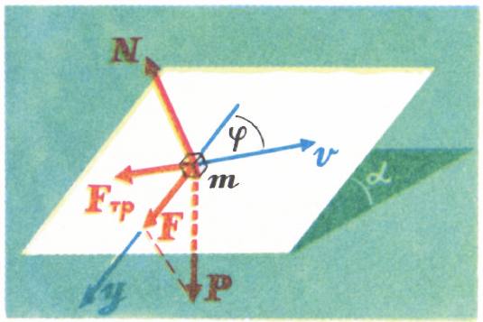
Fig. 8.

the fastest descent (y-axis) is affected by the gravity component F = mg sinα; in the direction opposite to the speed, the friction force F_tp = kN = kmg cosα acts. By condition, k = tanα, therefore F_tp = tanα kmg cosα = mg sinα = F.

Thus, the problem comes down to considering the movement of a cube under the influence of two forces of equal magnitude. One of them is always directed against the speed of the cube, the other along the y axis.

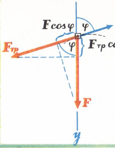
Fig. 9.

Let at some moment the speed v make an angle φ (Fig. 9) with the y axis. The tangential (direction tangent to the trajectory) acceleration a of the cube is determined by the force F_tp = F and the projection F cosφ of the force F to the same direction:

$$a = \frac{F + F \cos \varphi}{m}.$$

Acceleration a_y (along the y axis) is determined by the force F and the projection F_tp cosφ of the force F_tp onto the y axis. It is easy to see that the magnitude of this acceleration is equal to the tangential one:

$$a_y = \frac{F + F_tp \cos \varphi}{m} = \frac{F + F \cos \varphi}{m} = a.$$

Thus, the rate of change in the magnitude of the plane velocity a = \frac{\Delta v}{\Delta t} and the rate of change in the magnitude of the force component along the y axis a_y = \frac{\Delta v_y}{\Delta t} are the same. But if the rate of change in time of two quantities is the same, then these quantities themselves differ only by a constant that does not depend on time. Let us denote this constant by V. Then at any time v = v_y + V.

You can find the constant V by substituting the values ​​v and v_y into this formula

33

at the initial moment of movement of the cube ($v=v_0$, $v_y=v_0 \cos \beta$):

$$v_0 = v_0 \cos \beta + V.$$

From here

$$V = v_0 (1 - \cos \beta).$$

Hence,

$$v = v_y + v_0 (1 - \cos \beta),$$

Where

$$v_y = v \cos \varphi.$$

After a sufficiently long time, the “transverse” component of the cube’s speed will decrease to zero. The cube will move down along the $y$ axis. In this limiting state $\varphi = \pi$, that is $\cos \varphi = -1$; $v_y = -v$.

For steady speed $v$ we can write the equation

$$v = -v + v_0 (1 - \cos \beta).$$

From here

$$v = v_0 \frac{1 - \cos \beta}{2} = v_0 \sin^2 \frac{\beta}{2}.$$

Knowing that $a=a_y$, the problem can also be solved graphically. Indeed, if the change $\Delta v$ of the total speed is equal to the change $\Delta v_y$, then it is easy to find the values

$$v = v_0 \frac{1 - \cos \beta}{2} = v_0 \sin^2 \frac{\beta}{2}.$$

Knowing that $a=a_y$, the problem can also be solved graphically. Indeed, if the change $\Delta v$ of the total speed is equal to the change $\Delta v_y$, then it is easy to find the values

$$v = v_0 \frac{1 - \cos \beta}{2} = v_0 \sin^2 \frac{\beta}{2}.$$

Let after time $\Delta t$ the component $v_y$ of the speed of the cube changes to $\Delta v_y$, and the total speed - to $\Delta v = \Delta v_y$. Consequently, after time $\Delta t$ the vector $v_0$ will be $\Delta v$ shorter, and the value of its projection onto the $y$ axis changes by the same amount.

Through the point $B$, which lies below the point $A$ (the end of the vector $v_0$) to the segment $\Delta v_y = \Delta v$, we draw a horizontal line $BC$. With a radius $AB$ equal to $\Delta v_y = \Delta v$, draw arcs $BD$ from the point $A$ as from the center. The point $D$ will mark the length of the new vector $v = v_0 - \Delta v$. With a radius $OD$ equal to $v = v_0 - \Delta v$, draw an arc $DC$ from the point $O$ as from the center. The point $C$ of intersection of the arcs with the line $BC$ is the end of the desired vector $OC$, equal to $v$.

This construction can be done for any time intervals $\Delta t$. It shows that the velocity vector $v$ of the cube accelerates and approaches the axis $y$ (Fig. 11). From the drawing it is clear that in the limiting case

$$v + v_0 \cos \beta = v_0 - v.$$

From here

$$v = \frac{v_0 (1 - \cos \beta)}{2} = v_0 \sin^2 \frac{\beta}{2}.$$

The correct solution was sent by P. Belyakov (Moscow).

B. B. Bukhovtsev

34

F81

Currently, solenoids with superconducting windings are used. Such solenoids can create a magnetic field for a long time without consuming energy. However, if any section of the winding loses its superconducting properties, an accident will occur. In this area, more colic tella will be released and an explosion will occur.

Come up with the simplest device to prevent such accidents.

Schemes with relays are not suitable - their comparison time is too long. An explosion will occur before the relay trips. Therefore, the only way out is to short-circuit the solenode to resistance. This is how they usually do it. The wire for the solenoid is made reinforced with copper. If superconductivity is lost, the armature will serve as a buffer through which current appears, and the body release will be distributed throughout the circuit.

The correct solution was sent by S. Chernikov (Semipalatinsk). N. Efimov (Voronezh), V. Skvortsov (Leningrad).

F82

Find the conditions under which no current will flow through the resistance $r$ connected at points $A$ and $B$ of the circuit shown in figure 12.

So it will not go through resistance $r$ if the potential difference between points $A$ and $B$ is zero. Let us take the potential of point $F$ to be zero. then the potential of point $C$ is equal to $E_1$, and the potential of point $D$ is equal to $E_2$. Current $I = \frac{E_1}{r_1 + r_3}$ flows through resistance $r_1$,

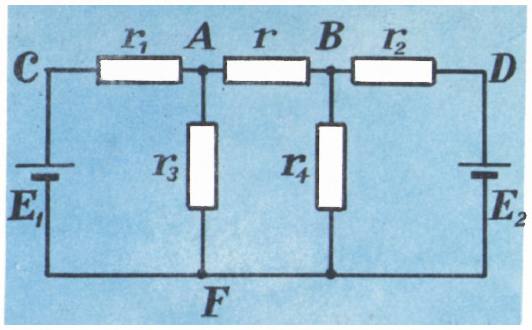
Fig. 12.

and therefore the voltage drop across resistance $r_1$ is equal to $U_1 = Ir_1 = E_1 \frac{r_1}{r_1 + r_3}$, and the potential of point $A$ is equal

$$\varphi_A = E_1 - E_1 \frac{r_1}{r_1 + r_3} = E_1 \frac{r_3}{r_1 + r_3}.$$

Similarly, we find the potential of point $B$:

$$\varphi_B = E_2 \frac{r_4}{r_2 + r_4}.$$

From condition $\varphi_A = \varphi_B$ we obtain

$$E_1 \frac{r_3}{r_3 + r_1} = E_2 \frac{r_4}{r_2 + r_4}.$$

This is the general condition for the absence of a point through resistance $r$. It also includes the very symmetrical case $r_1 = r_2$, $r_3 = r_1$ and $E_1 = E_2$.

I. Sh. Slobodetsky