Potential Energy Graphs

8

GRAPHICS
POTENTIAL
ENERGY

R. G. MINZ

How to find out whether body movement is limited and to what extent? Do equilibrium positions exist, and if so, are they stable or unstable?

In this article we will show that such questions are easy to answer if the potential energy of the body is known. We’ll discuss when it makes sense to talk about potential energy and how to calculate its magnitude at each point.

If we talk about potential energy, it means that we want to study the motion of a body, more precisely, of material points *), based on the law of conservation of mechanical energy.

This law states that for a closed system of material points (bodies) the quantities

$$E = T + U.$$

(1)

Sum

$$T = \frac{m_1 v_1^2}{2} + \frac{m_2 v_2^2}{2} + \dots + \frac{m_n v_n^2}{2}$$

is called the kinetic energy of the system, and $U$ is the potential energy of the interaction of the body. Kinetic energy in formula (1) reflects the body’s own motion, and potential energy, which depends on the distances between bodies, their mutual influence on each other.

In what follows, for simplicity, we will consider the movement only

*) As usual, by a material point we mean a body whose own dimensions in this problem are negligible.

one of the material points *), assuming that all the others are at rest. In such cases, we usually talk about the motion of a particle in an external strong field, and formula (1) takes the form

$$E = \frac{mv^2}{2} + U.$$

(2)

Speaking about the movement of a particle in an external field, we will consider the influence of stationary parts on moving ones, and all systems of parts as a whole are closed. There is, however, a subtlety to this. Let us trace it visually using the example of two materials of points with masses $m$ and $M$. Let a particle of mass $M$ dig around at some moment. Let us find out under what conditions it continues to remain motionless, that is, it will be possible to talk about the movement of a particle of mass $m$ in an external field. Let’s use the law of conservation of momentum

*) The problem of the movement of a large number of telecommunications interacting with each other is extremely complex. Until now, they had only been able to solve the problem of two bodies in a general form.

9

nia (after all, our system of bodies is closed): $M\vec{v} + m\vec{v}_1 = m\vec{v}_0$. (Here $\vec{v}_0$ is the initial speed of a particle with mass $m$, $v_1$ is its speed after some time and $v$ is the speed acquired by particles with mass $M$.)

Hence $\vec{v} = \frac{m}{M} (\vec{v}_0 - \vec{v}_1)$. If $\vec{v}_1 \neq \vec{v}_0$, then $\vec{v} = 0$ only when $M \to \infty$ Physical this means that $m \ll M$. Thus, the external field is the result of the action of heavy stationary particles on light ones. Let us recall two typical examples of an external field: a satellite in the Earth’s gravitational field, an electron in the field of a nucleus. In each of these examples, of course, condition $m \ll M$ is satisfied.

If the total energy $E$ of the particle is given, then correspondence (2) imposes restrictions on in which region of space the particle can be located. Indeed, after all, the kinetic energy $E_{\text{kin}} = \frac{mv^2}{2}$ allows on the basis of $\sqrt{\frac{2}{m}} E_{\text{kin}}$ to be minimal!), and from the law of conservation of energy it follows that

$$\frac{mv^2}{2} = E - U.$$

Thus, $E \geq U$; we have obtained a criterion for determining the region in which movement with total energy $E$ is possible. At points where $E = U$, kinetic energy, and therefore speed, vanishes.

Let us consider as an example the movement of a body along a straight line (axis $x$). Then the potential energy depends only on the position on this line: $U = U(x)$. In this case, our criterion is very convenient to apply graphically. Let us draw a straight line $U(x) = E$ on the horizontal potential energy graph. Wherever the potential energy graph passes below the straight line, $E > U$ and movement is possible. At the points of intersection, speed

10

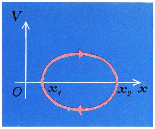
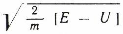
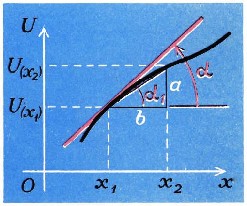
Fig. 2. The body, moving to the left, approaches the point $x_1$, where its speed is zero. One cannot accumulate at this point, since a force acts on it (see the sled rule on page 12). Therefore, it will continue to move to the right, increasing speed.

Knowing the potential energy, it is easy to determine the speed of the particle at each point. Since $\frac{mv^2}{2} = E - U$, then $v = \pm \sqrt{\frac{2}{m} [E - U]}$.

Two signs of speed correspond to two possible directions of movement along the $x$ axis. figure 2 graphically shows the dependence of the particle velocity on its position for the case when the energy and potential energy correspond to figure 1a. The direction of movement is indicated on the graph by an arrow.

So, we see that with the help of potential energy graphs we can simply and clearly find out where the possibility of movement is, what type of trajectories it has and how the speed of a body depends on its position. When clarifying these questions, we needed to know the behavior of potential energy as a function of coordinates “in general,” that is, how it behaves along the entire trajectory.

Let’s now see what is associated with the rate of change of potential energy, that is, the quantity

$$\frac{\Delta U}{\Delta x} = \frac{U(x_2) - U(x_1)}{x_2 - x_1},$$

where $\Delta x = x_2 - x_1$ is very small

According to the law of conservation of mechanical energy

$$\Delta U = U(x_2) - U(x_1) = \frac{mv_1^2}{2} - \frac{mv_2^2}{2} = \frac{m}{2} (v_1 + v_2) (v_1 - v_2)$$

where $v_1$ is the speed of the body at point $x_1$, and $v_2$ is its speed at point $x_2$. In a small area $\Delta x$ the force acting on the body can be considered constant. Movement under the influence of a constant force, which means $F$, equal to acceleration, and acceleration $a = F/m$. In this case, $v_2 - v_1 = a \Delta t = \frac{F}{m} \Delta t$ ($\Delta t$ is the time of movement), and $\frac{v_1 + v_2}{2}$ is equal to the average speed $\frac{v_1 + v_2}{2} = v_{cp} = \frac{\Delta x}{\Delta t}$. Let’s substitute these expressions into formula (4):

$$\Delta U = m \frac{\Delta x}{\Delta t} \left( -\frac{F}{m} \Delta t \right) = -F \Delta x.$$

From here

$$\frac{\Delta U}{\Delta x} = -F.$$

Formula (5) can also be obtained otherwise, taking into account that with uniform motion only the potential energy of the body changes and its change is equal to the work of the force acting on the body.

Let us find out the geometric meaning of formula (5). Let us be given a potential energy graph. It is clear that the smaller the value of $x_2 - x_1$, the more accurately the rate of change of potential energy coincides with the tangent of the tangent to the potential energy curve (Fig. 3). Action

11

Indeed, $tg\alpha_1 = \frac{a}{b} = \frac{U(x_2) - U(x_1)}{x_2 - x_1}$, and the smaller $x_2 - x_1$, the more accurately the angle $\alpha_1$ is equal to the angle $\alpha$. Thus, we come to the conclusion that the tangent of the tangent to the potential energy graph, taken with the opposite sign, coincides with the force acting on the body. This means that the more the potential energy increases, the greater the magnitude of the force and vice versa.

After formula (5) has acquired a clear geometric meaning, it is easy, for example, to find out whether equilibrium positions exist and what they are. We call the equilibrium position the point at which a body can remain for as long as possible, provided, of course, that it initially has zero speed. When is this possible? A change in speed is characterized by acceleration: if it is zero, then the speed of the body is unchanged. Acceleration is proportional to the force acting on the body. This means that equilibrium positions are those points where the force vanishes.

Let’s look again at the potential energy graph. As we have already seen, the force acting on a body is equal to the tangent of the tangent to the potential energy curve taken with the opposite sign. If this angle is zero, then the force is zero. Thus, on the potential energy graph, the equilibrium positions correspond to those points at which

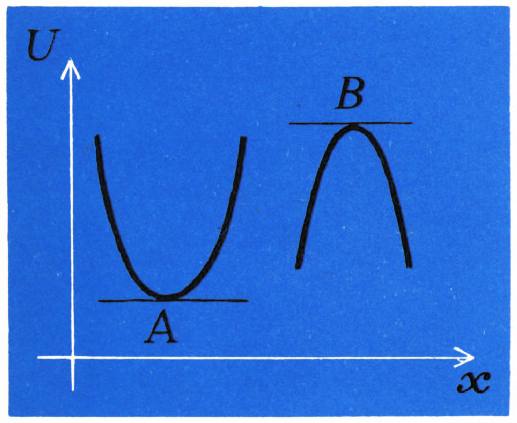
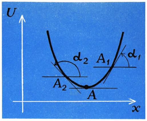
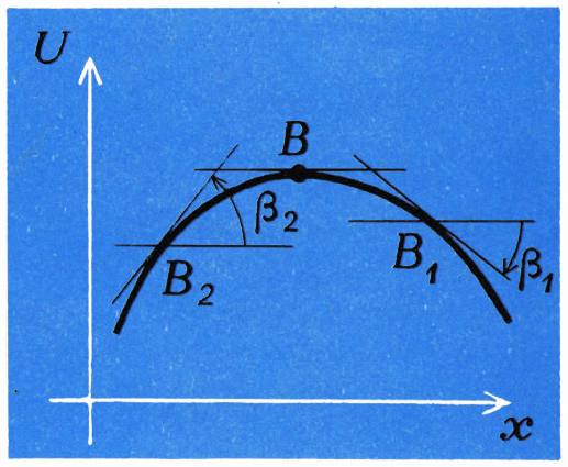
Fig. 4

Fig. 5a,6

whose tangent is parallel to the abscissa axis. It is obvious, for example, that equilibrium positions are maxima and minima of potential energy (Fig. 4).

Equilibrium positions can be stable and unstable. What do you mean? Let us slightly deviate the body from its equilibrium position. If at the same time the force acting on the body returns it back, then the equilibrium is called stable; if not, then it is unstable.

Let us examine for stability the equilibrium position corresponding to the minimum on the potential energy curve (point $A$ on Fig. 4). Let the body move from point $A$ to the right. In the new position $A_1$ (Fig. 5 a), the tangent of the tangent angle is positive, and the force is negative, that is, directed in the direction opposite to the displacement and returns the body to

12

point $A$. If you should merge to the left of point $A$, then in this position ($A_2$ on Fig. 5 a) the tangent of the tangent angle is negative, the force is positive, that is, directed to point $A$ and forces the body to return to its original position. Thus, the equilibrium position at the minimum potential energy is stable. Similarly, we can consider the stability of the equilibrium position if the potential energy is maximum (Fig. 5 b).

So, we see that from the potential energy curve we can find the magnitude of the force acting on the body, and it is easy to determine where the equilibrium positions are and what they are. In this sense, the potential energy graph can be compared to an ice slide from where it descends to the Sankh. In those places where the hill is round, the sled accelerates quickly; on a gentle descent, it accelerates more slowly. The top of the slide and the depressions in it are the equilibrium positions. After all, if you put a sled there, they will stay there. In this case, the top is the position of unstable equilibrium, and the valley is stable.

Now, perhaps, let’s talk about how to calculate the value of potential energy. To do this, let us return again to formula (5) and rewrite it in the form

$$U(x_2) - U(x_1) = -F \cdot (x_2 - x_1).$$

Recall that the length $\Delta x = x_2 - x_1$

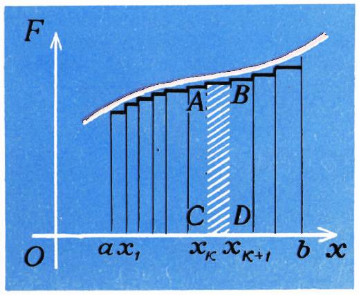
Fig. 6

13

The energy of the body is equal to the area taken with the opposite sign *) under the graph of the dependence of the action of force on the body on the coordinates **). Then its graph is a straight line parallel to the x-axis. The area under it is equal to $F \cdot (x - x_0)$, from where we obtain for the difference in potential energies

$$U(x) - U(x_0) = -F \cdot (x - x_0)$$

(Fig. 7a, b).

Using correspondence (8) we obtain

$$\frac{mv^2}{2} - \frac{mv_0^2}{2} = F \cdot (x - x_0).$$

$$\frac{mv^2}{2} - Fx = \frac{mv_0^2}{2} - Fx_0,$$

that is, potential energy $U = -Fx$. However, this is not the only possibility; with the same reason we could write such an equality

$$\frac{mv^2}{2} - Fx + C = \frac{mv_0^2}{2} - Fx_0 + C,$$

where $C$ is a constant number. But then the potential energy is $U = -Fx + C$. Thus, we see that the potential energy is determined exactly up to an arbitrary constant. This can be explained by the very law of conservation of mechanical energy. After all, if we say that the quantities $E = \frac{mv^2}{2} + U$ are conserved, then $E' = \frac{mv^2}{2} + U + C$ is also conserved, where $C$ is some constant. But in this case $U' = U + C$. This means that potential energy can only be determined to an accuracy of an arbitrary constant, which is always chosen from messages of convenience *). Of course, such uncertainty of potential energy does not in any way affect the conclusions we have drawn about the characteristics of motion in a given field, the presence of equilibrium positions in it, and the dependence of the body’s speed on the coordinate. You can easily verify this; you only need to simultaneously change the potential energy by values ​​$C$ and change the total energy of the body by the same amount. The fact is that to fully describe the movement of a body, it is necessary to specify its position and speed at some moment

*) It should be noted that if the force is negative, then the corresponding participation should be assigned a minus sign.

*) A field in which the force acting on the body is constant everywhere is called homogeneous. Homogeneous, for example, is the gravitational field near the Earth’s surface $F = mg$ and the electric field inside a flat capacitor.

14

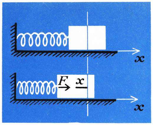
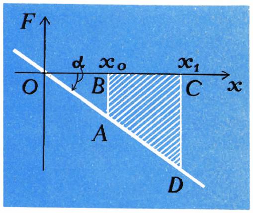
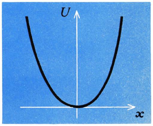
Fig. 8

time, thereby we will know
$\frac{mv_0^2}{2}$ and $U(x_0)$ Polyana energy
$E = \frac{mv_0^2}{2} + U(x_0)$ By adding some constant value to $U$, the energy of $E$ will increase by exactly the same amount.

Let us now consider the motion of the cube outside in the absence of friction (Fig. 8) and calculate what the potential energy is in this case. According to Hooke’s law, the force acting on the cube is equal to $F = -kx$, where $k$ is the stiffness of the spring $x$ is its deformation. In this case, the graph of the force is straight, the tangent of the angle of inclination of which to the axis $x$ equals $k$ (Fig. 9a)

The potential energy difference $U(x_1) - U(x_0)$ is equal to the area of ​​the trapezoid $ABCD$ protected on Fig. 9a, the height of which is $BC = x_1 - x_0$. and we get the main $\frac{AB + CD}{2} = \frac{kx_0 + kx_1}{2}$. Using the formula for the area of ​​a trapezoid, we find that $U(x_1) - U(x_0) = \frac{(x_1 - x_0)(kx_0 + kx_1)}{2} = \frac{k(x_1^2 - x_0^2)}{2} = \frac{kx_1^2}{2} - \frac{kx_0^2}{2}$.

As a result, for $U(x)$ we obtain the following expression: $U(x) = \frac{kx^2}{2}$

*) Similar to the case of a homogeneous field with constant $C$, we chose here so that $U(0) = 0$.

15

cases ($F = \text{const.} \quad F = -kx$) it is impossible to calculate this area without knowledge of integral calculus. If we find it, then it turns out that for a force changing according to the law $F = \frac{\alpha}{r^2}$, the potential energy

$$U = \frac{\alpha}{r}$$

Please note that in formula (10) we have chosen the constant $C$ so that the potential energy vanishes at infinity. Why is this convenient and when? Let us remember that potential energy characterizes the action of bodies on each other—interaction; if at infinity the force becomes zero, then the further the bodies are separated from each other, the weaker their mutual influence. This is precisely why the choice of constant in our and similar ($F(\infty) = 0$) cases is accordingly.

From formula (10) it follows that the type of potential energy significantly depends on the sign of $\alpha$ (see Fig. 106). If $\alpha > 0$, then the force is $F = \frac{\alpha}{r^2} > 0$, and we are dealing with repulsion (like charges, $\alpha = q_1 q_2 > 0$). If $\alpha < 0$, then the force is $F = -\frac{|\alpha|}{r^2} < 0$, which corresponds to attraction (opposite charges, $\alpha = -q_1 |q_2|$). Here, please, it is worth returning once again to the analogy with a sled going down an ice slide. Notice that if you put a sled on a slide that has a potential energy interwash profile, they point in the direction of the force. Such a set of rules makes it possible to immediately determine whether attraction or repulsion is taking place. Indeed, if the sank is shown to the point $r = 0$ (for example, the lower curve at Fig. 106), then attraction takes place, if on the contrary (for example, the upper curve), then repulsion occurs.

The same rule allows us to qualitatively construct the type of potential

16

Stifling. At large distances, attraction quickly kills, and recoil when approaching, starting from a certain distance, returns very sharply. The described picture of the interaction of atoms corresponds to the potential energy graph. Shown-

16

nyy on figure 11 Make sure of this, use the analogy with an ice slide. Point $r=r_0$ corresponds to the position of stable equilibrium, and therefore $r_0$ is equal to the distance between atoms in the molecule.

In conclusion, let us summarize some results. We have seen that from the potential energy graph we can find out a number of essential characteristics of movement (the number of different trajectories depending on the energy, whether the movement is limited or not, whether there are equilibrium positions and whether they are stable or unstable). Each of them, as it turned out, has a simple geometric meaning. It is also easy to determine the magnitude and direction of the force acting on the body (“the sled rule”). We have shown that the area under the force graph, taken with the opposite sign, is equal to the potential energy of the body. This makes it possible in some cases to directly calculate potential energy. This makes solving various problems much easier.

And finally, we have seen how the qualitative form of potential energy allows us to understand what exists and give an answer to it.

Now try to solve the following problems yourself.

Exercises

1. Find out the area of ​​possible movement when
   $E<U_0$ and $E>U_0$.
   if the potential energy has the form shown in Fig. 12.

2. Find equilibrium positions along the potential energy curve (Fig. 13) and find out their stability.

Draw a graph of force versus coordinate.

3. Show geometrically that when the potential energy changes by a constant value $C$, the force acting on the body at each point does not change.

4. A cube with side $a$ of density $\rho_1$ floats on the surface of a liquid whose density is $\rho_2$. Draw graphs of the force acting on the cube and the potential energy depending on the depth of the piercing.