Experiments with pendulums

26

LABORATORY “QUANTA”
with EXPERIENCES
PENDULUM
G.L.Kotkin

It is difficult to find physical devices that were as simple in design and reliable in use as matnikki. Meanwhile, experiments with them can lead to interesting results, which are extremely important not only in mechanics, but also in radio engineering and electrical engineering. Try to do the suggested experiments yourself and explain the effects that you will observe. Although the experiments themselves are very simple, however, it is not easy to fully understand the increase in matniki: for this you need to know the basic laws of harmonic vibrations and have experience in trigonometric transformations. Apparently, only tenth graders will be able to fully understand this article, but schoolchildren in grades 8-9 can carry out these experiments and fully explain them, at least qualitatively.

Matnik with suspension division

Make a mat with a split hanger, shown at figure 1. The length of the mat $l$ should be much longer than the length of the top divided part of the hanger.

Push the mat at an angle to the figure plane. You will see that at first the matnik will be qualitatively in the direction only, but soon its movement will turn into rotation in the circle of the vertical axis. Then the mat will begin to oscillate again in the plane, but no longer in the one in which it was pushed. After this, the rotation will begin again, but in the other direction. Gradually it will be replaced by movement in the direction of the first oscillatory shock. Then everything will repeat again from the beginning.

What is the reason for this behavior of the matnik?

Related matniki

a) Two identical mats (for example, nuts on a thread) will be hung on a not very tight stretched thread $AB$ (Fig. 2). Reject one of the matniks and release.

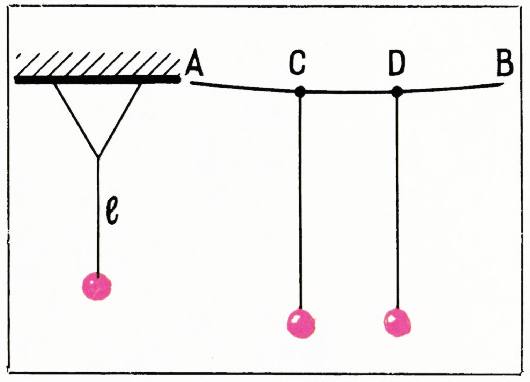
Fig. 1. Fig. 2.

27

Try changing the weights of the weights, changing the lengths of the threads of the mats, and the tension of the upper thread.

6. Attach two matrices to the rigid frame. Then tie the threads of the matniks with a thread at a certain height (Fig. 3). Reject one of the mats and lower it. Look how the matniki will move.

Double matnik

The structure of the double matnik is shown in figure 4. The upper weight is much heavier than the lower one, and the long threads are the same. Push the bottom weight and watch it move.

Let’s now understand the behavior of these matniks.

1. Let’s start with a matnik with an unlinked suspension.

The rather complex behavior of the matnik that you observe can be explained by the fact that its movement consists of two oscillatory movements (Fig. 5): parallel to the plane $zy$ and perpendicular to it. These oscillations occur independently of each other (if the deviations of the mat from the vertical are not too large), and the periods of their corresponding ones are equal

$$T_1 = 2\pi \sqrt{\frac{l}{g}} \quad T_2 = 2\pi \sqrt{\frac{L}{g}}.$$

First of all, let’s learn how to describe the movement of a weight using coordinates.

Let the point $A$ move along a circle of radius $a$ with an angular velocity $\omega$ counterclockwise (Fig. 6a) or clockwise (Fig. 66). Then the projection $B$ of the point $A$ onto the axis $x$ performs a harmonic oscillation*) with an angular frequency $\omega$ equal to $\frac{2\pi}{T}$ and an amplitude $a$.

The projection $C$ of the same point $A$ onto the axis $y$ makes similar oscillations, but reaches its maximum deviation from point $O$ a quarter of a period later - after the time during which the radius $OA$ makes $\frac{1}{4}$ revolutions around the point $O$. It is easy to verify this by following the movements of points $C$ and $B$ when rotating the radius $OA$. At the moment when the projection of the point $A$ onto the axis $x$ is maximally deviated from the point $O$, its projection onto the axis $y$ is just

*) See, for example, the article by Ya. A. Smorodinsky “Similar movements”, «Kvant» No. 9, 1971.

29

direction $OD$ (Fig. 7) to a distance $a$ and then release, then the coordinates of the weight will change according to the formulas:

$$\begin{cases} x = a \cos \omega_1 t, \\ y = a \cos \omega_2 t, \end{cases}$$

Where

$$\omega_1 = \frac{2\pi}{T_1} = \sqrt{\frac{g}{l}},$$

$$\omega_2 = \frac{2\pi}{T_2} = \sqrt{\frac{g}{L}},$$

$$a = \frac{b}{\sqrt{2}}.$$

Recall that $l$ and $L$ have very little difference from each other, that is, the frequencies of $\omega_1$ and $\omega_2$ are almost the same. Therefore, at first, oscillations along the $x$ and $y$ axis will occur almost in phase.

Since $\omega_1 > \omega_2$, over time the oscillation along the $y$ axis lags behind the oscillation along the $x$ axis more and more. But, as we have seen, when a point moves counterclockwise around a circle, the oscillations of its projections on the $x$ and $y$ axes lag behind each other by the fourth period. It follows that when the lag of the oscillations of the weight along the axes $x$ and $y$ reaches the fourth period, it will move just along the circle counterclockwise. When the oscillations of the weight lag along the axes $x$ and $y$ on the field of motion, it will move along the straight line $E'D'$. Then the lag of the oscillation along the $y$ axis will reach the $\frac{3}{4}$ period - the weight moves around the circle clockwise. Finally, when there is a delay of an entire period, the weight again oscillates along the straight line $ED$. This is what you observed.

It is convenient to “retell” these wonders using formulas. System (5) can be represented as

$$\begin{cases} x = a \cos \omega_1 t, \\ y = a \cos (\omega_1 t - \phi), \end{cases}$$

where $\phi = (\omega_1 - \omega_2) t$. Over two or three periods, $\phi$ remains almost unchanged, but over many periods it increases steadily. For $\phi = 0, \frac{\pi}{2}, \pi, \frac{3\pi}{2}$, formulas (6) coincide in sequence with formulas (3), (1), (4), (2).

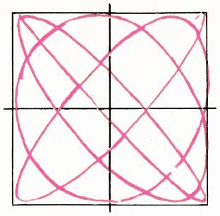
Fig. 9.

At $\phi = 2\pi$ the weight returns to motion in a straight line $ED$.

The stated theory can be tested experimentally. After all, we can calculate how long it will take for the weight to move through the entire cycle of changes. If it is time $T_0$, then $\phi_0 = (\omega_1 - \omega_2) T_0 = 2\pi$, opening $\frac{2\pi}{T_0} = \omega_1 - \omega_2$, or

$$\frac{1}{T_0} = \frac{1}{T_1} - \frac{1}{T_2}.$$

Now you need to measure the oscillation periods $T_1$ and $T_2$ of the pendulum, then in the $yz$ plane, another time in the $xz$ plane. Time $T_0$ is measured independently. After measuring $T_1$, $T_2$ and $T_0$, check the correctness of formula (7). To measure $T_1$ and $T_2$ it is better to determine the time, say, in 10-15 vibrations. It is immediately revealed what reasons lead to deviations from the calculation. Apparently, the damping of oscillations caused by air resistance is primarily affected. Well, the weights shouldn’t be too light.

In reality, the movements will not occur in a straight line or circle, but along a complex trajectory. This trajectory (Fig. 9) more or less uniformly “fills” the entire square.

If the initial angle with the symmetry plane is different from $\frac{\pi}{4}$, then the characteristic “instantaneous” trajectories of the weight are the diagonals of the right angle and the ellipses inscribed in it.

The fact that the movement of the pendulum consists of independent oscillations is expressed by saying that the superposition principle is valid for its oscillations *).

2. Let’s move on to explaining the movement of the connected pendants (Fig. 2 and 3). If we deflect and then release one of them, we will see that the other will gradually begin to move.

*) Reader «Kvant» have already encountered the principle of superposition when explaining the type of wave on the surface of water («Kvant» No. 1, 1971, p. 32).

30

This is explained by the fact that when the first matrix is ​​deflected by the bond, their thread is deformed and the elastic force acts on the other matrix, imparting acceleration to it. The first matrix will oscillate with less and less amplitude and finally stop. At this time, the amplitude of vibrations of the second matrix will be the most magnificent. Then the first matrix will roll out, and the second will stop, and so on.

The complex oscillatory motion of a system consisting of two matrices can be represented as the result of the addition (superposition) of two oscillations with frequencies $\omega_1$ and $\omega_2$. One of the frequencies is equal to the frequency with which both matrices will oscillate if they are simultaneously deflected in one direction and then released (Fig. 10). Let’s denote this frequency by $\omega_1$. Another frequency is $\omega_2$. This is the frequency with which both matrices will vibrate if they are first simultaneously deflected in opposite directions and then released (Fig. 11).

Note that the angular frequency $\omega_2$ is greater than the angular frequency $\omega_1$. These two vibrations are called normal vibrations of two coupled matrices.

Let’s write the equation of normal vibrations. First

$$\begin{cases} x_1' = a \cos \omega_1 t, \\ x_2' = -a \cos \omega_1 t, \end{cases}$$

second

$$\begin{cases} x_1'' = a \cos \omega_2 t, \\ x_2'' = a \cos \omega_2 t. \end{cases}$$

Let’s add the mixtures $x_1'$ with $x_1''$ and $x_2'$ with $x_2''$. We get:

$$\begin{cases} x_1 = x_1' + x_1'' = a \cos \omega_1 t + a \cos \omega_2 t, \\ x_2 = x_2' + x_2'' = -a \cos \omega_1 t + a \cos \omega_2 t. \end{cases}$$

Using the formula for adding cosines, we get:

$$\begin{cases} x_1 = A \cos \Omega t, \quad \Omega = \frac{\omega_1 + \omega_2}{2}, \\ A = 2a \cos \left( \frac{\omega_1 - \omega_2}{2} t \right). \end{cases}$$

Due to the fact that $\omega_1$ differs little from $\omega_2$, the expression $\cos \left( \frac{\omega_1 - \omega_2}{2} t \right)$ is close to 1 (if $\omega_1$ is equal to $\omega_2$, then this expression is equal to 1). Therefore, it has little effect on the value of $x_1$. Therefore, the factor $2a \cos \left( \frac{\omega_1 - \omega_2}{2} t \right)$ in the expression for $x_1$ can be considered as slowly changing the amplitude (red point on Fig. 12, a). The situation is similar